Long vs Wide Data Formats

AlgebraOfGraphics works with both long and wide data formats. Understanding the difference helps you choose the right approach and write clearer plotting code.

What is Long Format?

In long format (also called "tidy" format), each row represents one observation. If you have multiple groups or categories, they're indicated by values in a categorical column rather than spread across separate columns.

Here's an example of long format data:

x	y	group
1	1.0	y1
2	1.5	y1
1	1.1	y2
2	1.6	y2

Long format is the most convenient for AlgebraOfGraphics. Mappings are straightforward because you just reference column names directly:

mapping(:x, :y, color = :group)

What is Wide Format?

In wide format, multiple related measurements are spread across different columns. This is often how data comes naturally from experiments, spreadsheets, or measurement devices.

The same data in wide format:

x	y1	y2
1	1.0	1.1
2	1.5	1.6

Wide format can be used with AlgebraOfGraphics, but requires more complex multidimensional mappings. You specify a vector of column names and use helpers like dims() to create categorical groupings.

Converting Between Formats

You can convert between formats using DataFrames functions.

Wide to Long (using stack):

using DataFrames

# Wide format
df_wide = DataFrame(x = [1, 2], y1 = [1.0, 1.5], y2 = [1.1, 1.6])

# Convert to long format
df_long = stack(df_wide, [:y1, :y2])
rename!(df_long, :value => :y, :variable => :group)

4×3 DataFrame

Row	x	group	y
	Int64	String	Float64
1	1	y1	1.0
2	2	y1	1.5
3	1	y2	1.1
4	2	y2	1.6

Long to Wide (using unstack):

# Long format
df_long = DataFrame(x = [1, 2, 1, 2], y = [1.0, 1.5, 1.1, 1.6], group = ["y1", "y1", "y2", "y2"])

# Convert to wide format
df_wide = unstack(df_long, :x, :group, :y)

2×3 DataFrame

Row	x	y1	y2
	Int64	Float64?	Float64?
1	1	1.0	1.1
2	2	1.5	1.6

Plotting with Long vs Wide Format

Let's see how the same plots look with each format. We'll use a practical example with multiple y-values for each x:

using AlgebraOfGraphics, CairoMakie, DataFrames

# Wide format
df_wide = DataFrame(x = 0.0:10)
for i in 1:5
    df_wide[!, "y$i"] = df_wide.x .^ (0.4 + i * 0.1)
end
ys = names(df_wide, Not(:x))

# Long format
df_long = stack(df_wide, ys, variable_name = :group, value_name = :y)

Example 1: Lines without color differentiation

Wide format:

data(df_wide) * mapping(:x, ys) * visual(Lines) |> draw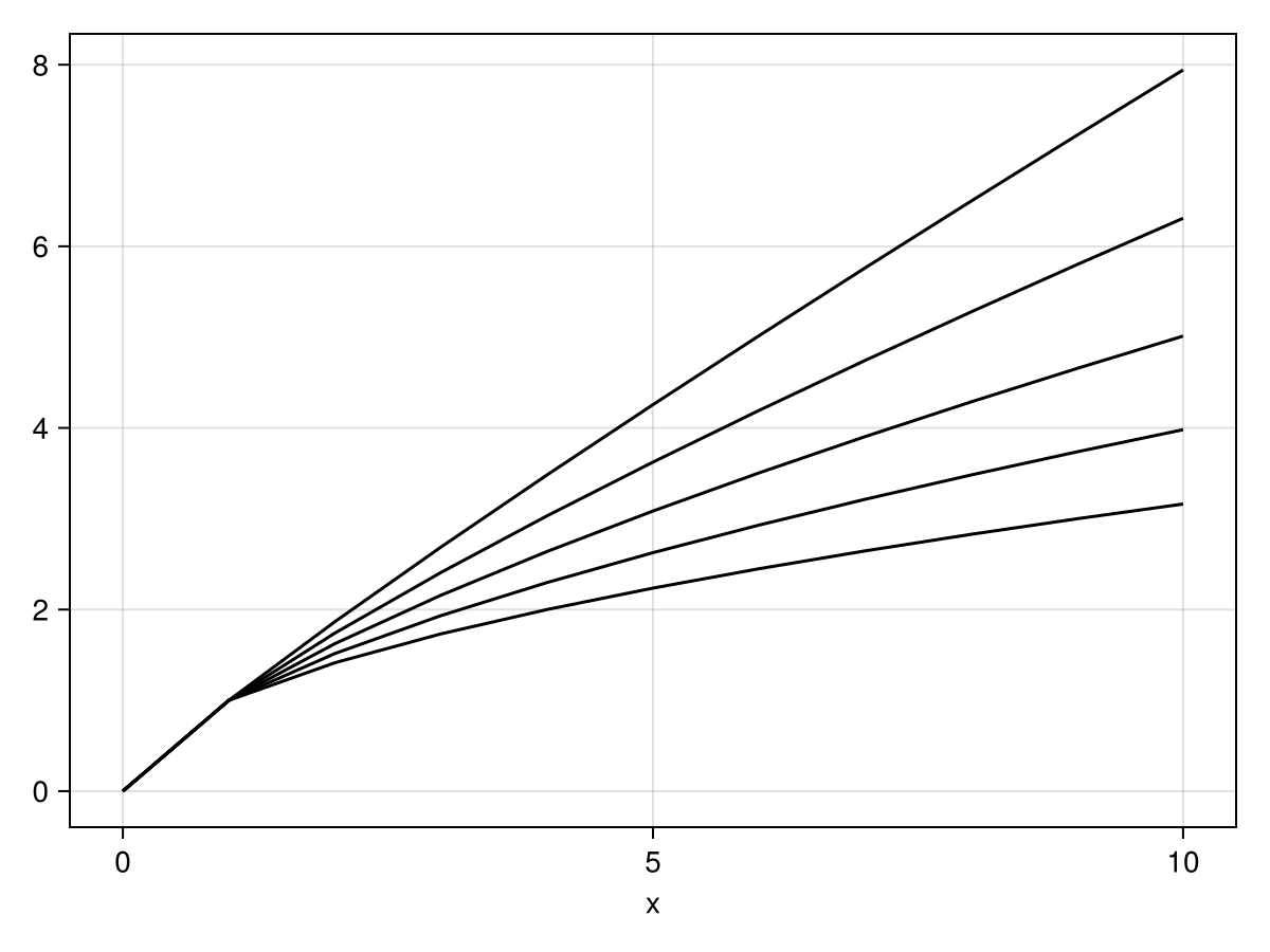

Long format:

data(df_long) * mapping(:x, :y, group = :group) * visual(Lines) |> draw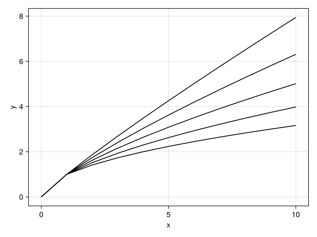

In long format, we need the group mapping to create separate lines. Without it, all points would connect into one zigzagging line.

Example 2: Lines differentiated by color

Wide format:

data(df_wide) * mapping(:x, ys, color = dims(1)) * visual(Lines) |> draw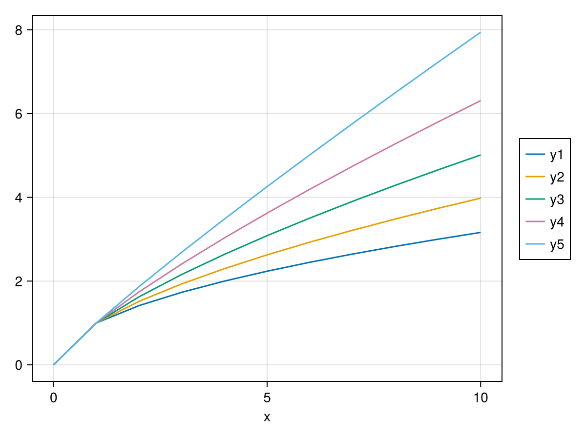

Long format:

data(df_long) * mapping(:x, :y, color = :group) * visual(Lines) |> draw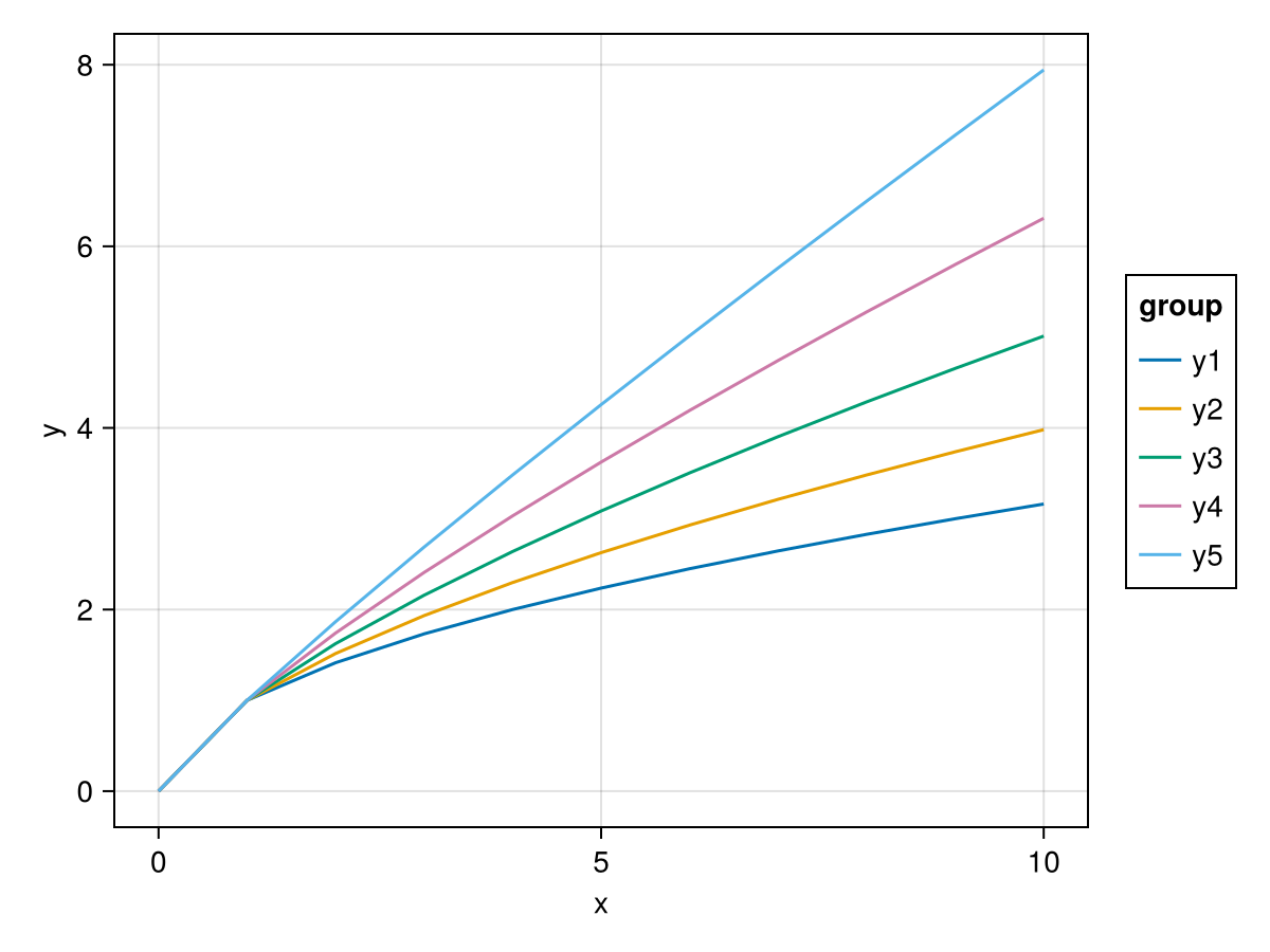

Notice how the long format version is a bit simpler: just color = :group. The wide format uses dims(1) to create a categorical variable from the first dimension, the column labels are automatically used as labels of the categorical values that dims creates. Because there are two different y-labels, the y axis doesn't have a label by default in wide mode.

Example 3: Custom color palette

Wide format:

data(df_wide) * mapping(:x, ys, color = dims(1)) * visual(Lines) |>
    draw(scales(Color = (; palette = :Set1_5)))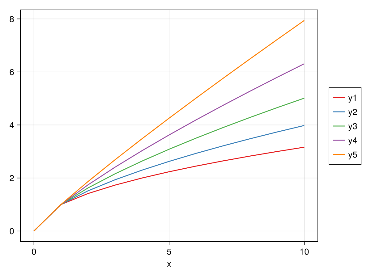

Long format:

data(df_long) * mapping(:x, :y, color = :group) * visual(Lines) |>
    draw(scales(Color = (; palette = :Set1_5)))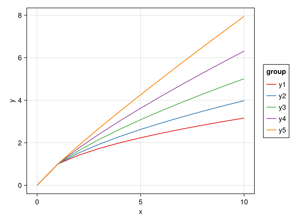

The scales function works the same way for both formats.

Example 4: Lines differentiated by style

Wide format:

data(df_wide) * mapping(:x, ys, linestyle = dims(1)) * visual(Lines) |> draw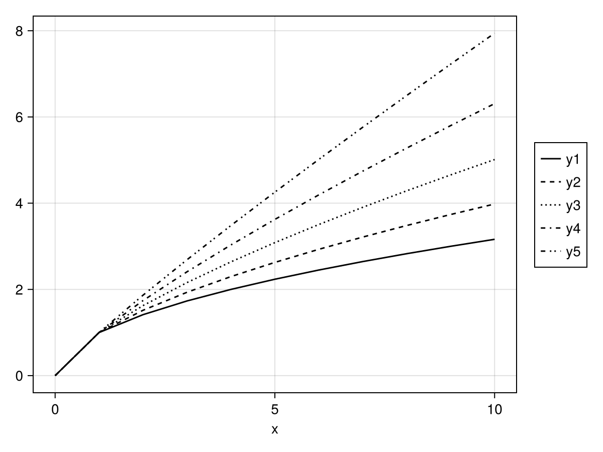

Long format:

data(df_long) * mapping(:x, :y, linestyle = :group) * visual(Lines) |> draw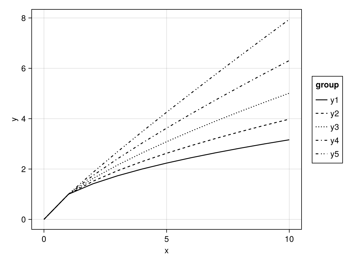

Example 5: Scatter plot with color

Wide format:

data(df_wide) * mapping(:x, ys, color = dims(1)) * visual(Scatter) |> draw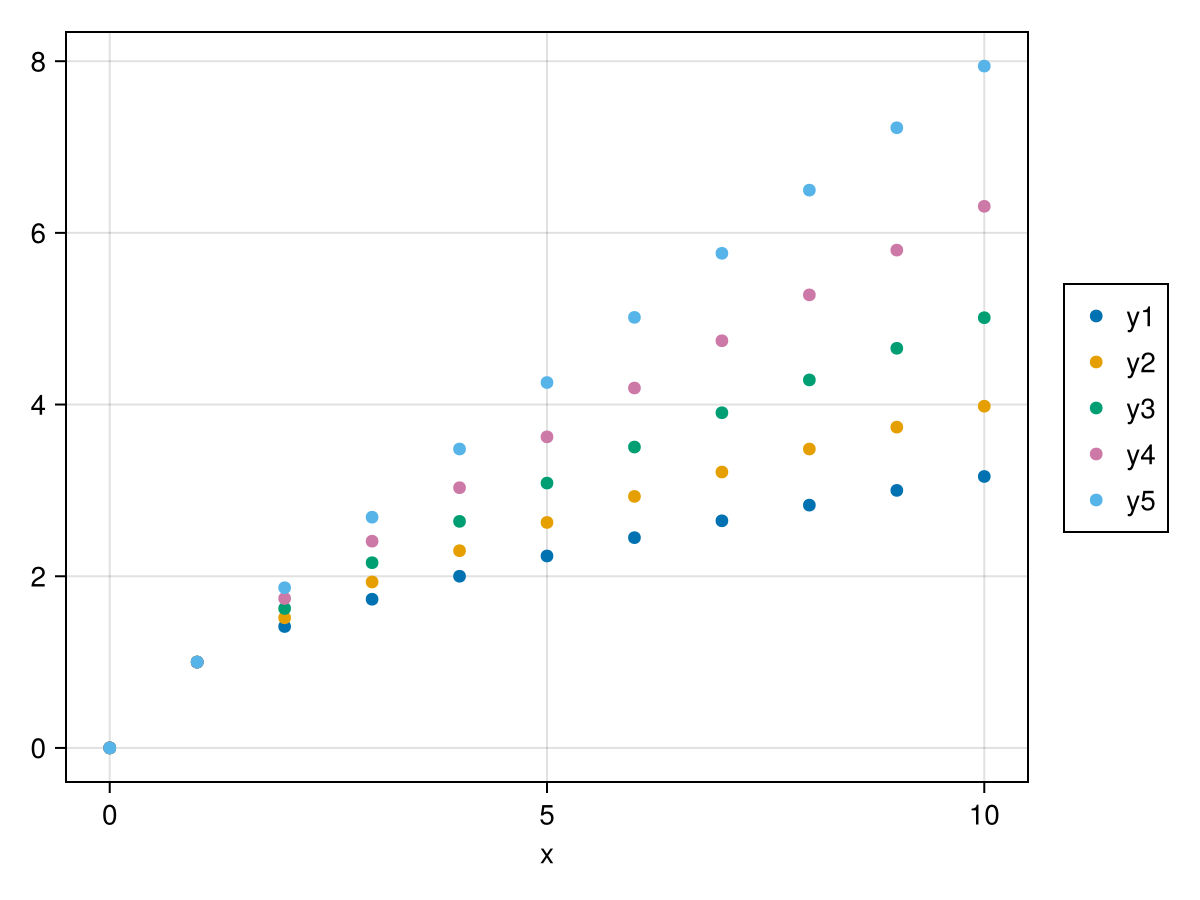

Long format:

data(df_long) * mapping(:x, :y, color = :group) * visual(Scatter) |> draw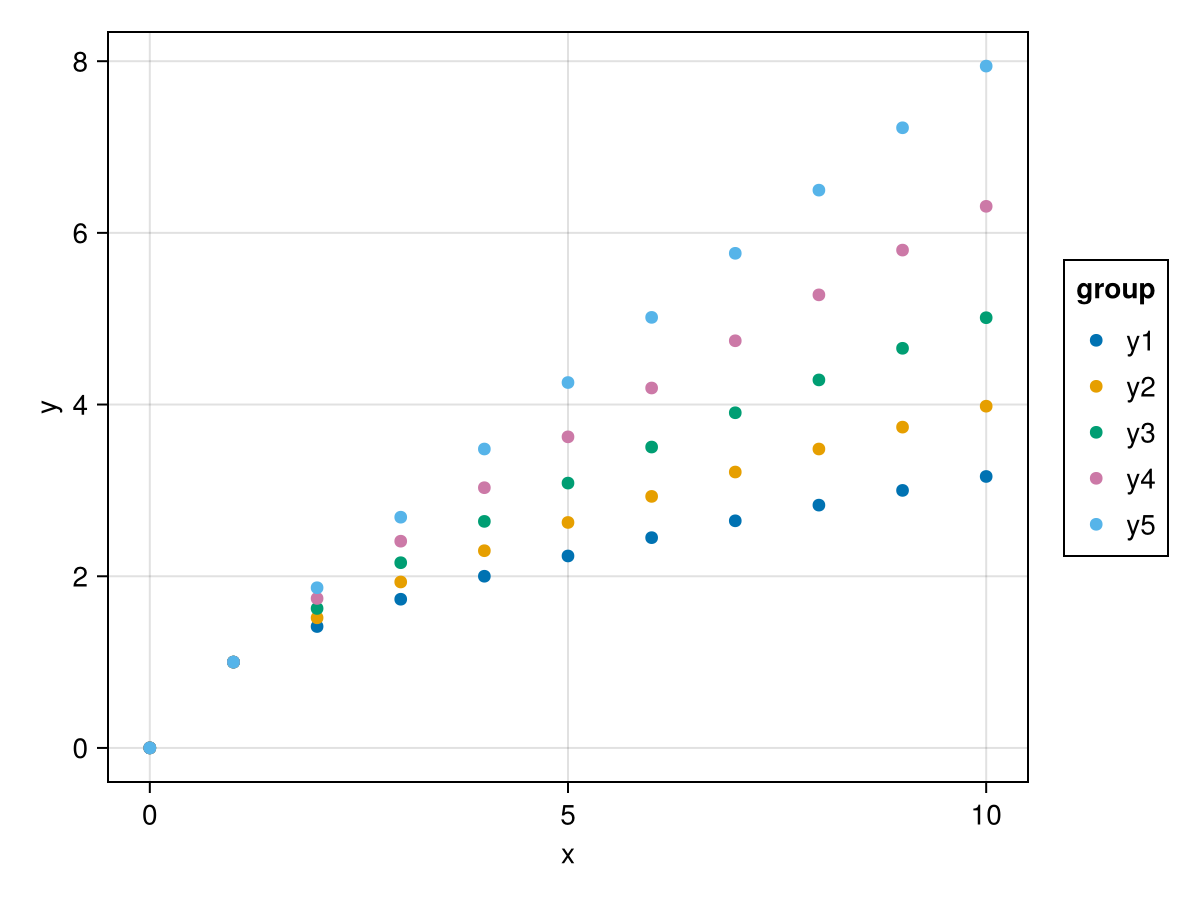

Example 6: Scatter plot with different markers

Wide format:

data(df_wide) * mapping(:x, ys, marker = dims(1)) * visual(Scatter) |> draw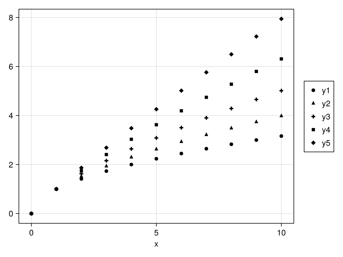

Long format:

data(df_long) * mapping(:x, :y, marker = :group) * visual(Scatter) |> draw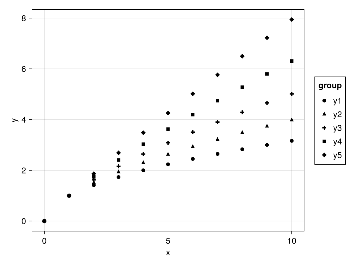

Understanding Wide Format Mappings

When you use wide format, you're creating a multidimensional mapping. Each element of the array gets processed through the full grouping pipeline.

In the example mapping(:x, ys) where ys = ["y1", "y2", "y3", "y4", "y5"], you're creating a one-dimensional array with 5 elements. These elements refer to columns of the data, and each column becomes a separate trace in the plot.

The dims(1) helper creates a categorical variable along the first dimension of this array. This is what allows you to map that dimension to aesthetics like color or linestyle. The column labels are automatically used as category labels in legends and other visual elements.

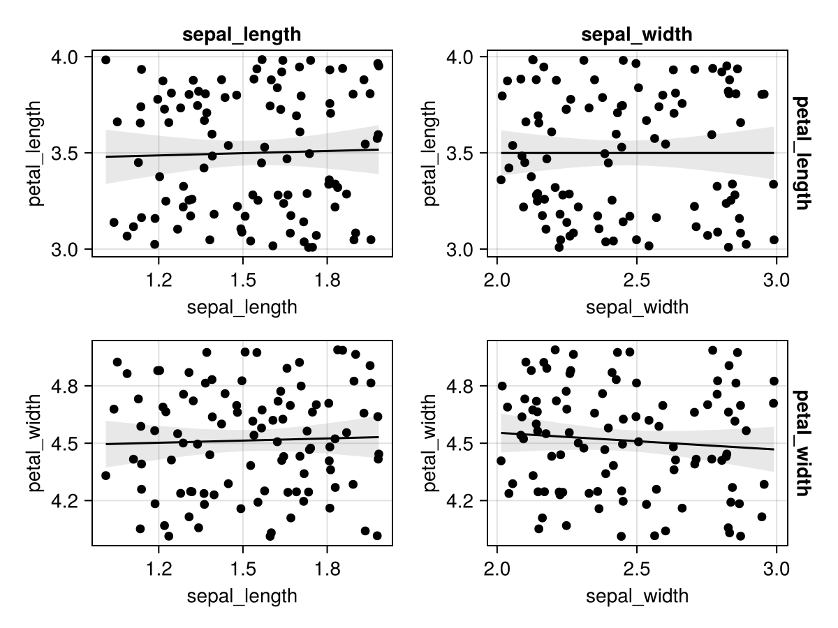
Faceting and axis linking with wide data

When using wide format with faceting, AlgebraOfGraphics links only those axes that have the same label:

df_facet = (
    sepal_length = 1 .+ rand(100),
    sepal_width = 2 .+ rand(100),
    petal_length = 3 .+ rand(100),
    petal_width = 4 .+ rand(100)
)
xvars = ["sepal_length", "sepal_width"]
yvars = ["petal_length" "petal_width"]
layers = linear() + visual(Scatter)
plt = data(df_facet) * layers * mapping(xvars, yvars, col=dims(1), row=dims(2))
draw(plt)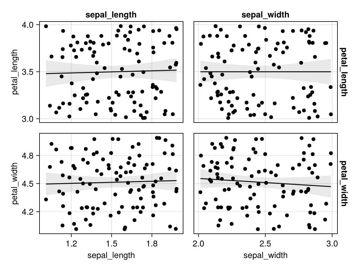

You can control axis linking behavior:

draw(plt, facet = (; linkxaxes = :all, linkyaxes = :all))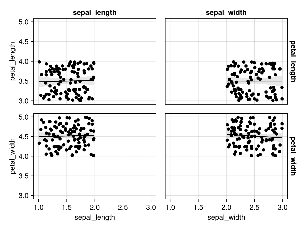

draw(plt, facet = (; linkxaxes = :none, linkyaxes = :none))