Frequently Asked Questions
What is the algebraic structure of AlgebraOfGraphics?
AlgebraOfGraphics is based on two operators, + and *. These two operators induce a semiring structure, with a small caveat. Addition is commutative only up to the drawing order. For example, visual(Lines) + visual(Scatter) is slightly different from visual(Scatter) + visual(Lines), in that the former draws the scatter on top of the lines, and the latter draws the lines on top of the scatter. As a consequence, only right distributivity holds with full generality, whereas left distributivity only holds up to the drawing order.
Why is the mapping pair syntax different from DataFrames?
The transformations passed within a mapping, e.g. mapping(:x => log => "log(x)"), are applied element-wise. Operations that require the whole column are not supported on purpose. An important reason to prefer element-wise operations (other than performance) is that whole-column operations can be error prone in this setting, especially when
the data is grouped or
different datasets are used.
If you do need column-wise transformations, consider implementing a custom analysis, such as density, which takes the whole data as input, or apply the transformation directly in your data before passing it to AlgebraOfGraphics.
See also Pair syntax for a detailed description of the pair syntax within a mapping.
What is the difference between axis scales and data transformations?
There are two overlapping but distinct ways to rescale data.
Keep the data as is and use a nonlinear scale, e.g.
axis=(xscale=log,).Transform the data directly, e.g.
mapping(:x => log => "log(x)").
Note that the resulting plots may "look different" in some cases. Consider for instance the following example.
using AlgebraOfGraphics
using AlgebraOfGraphics: density
df = (x = exp.(randn(1000)),)
kde1 = data(df) * mapping(:x) * density()
draw(kde1, axis=(width=225, height=225, xscale=log,))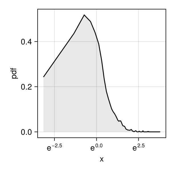
df = (x = exp.(randn(1000)),)
kde2 = data(df) * mapping(:x => log => "log(x)") * density()
draw(kde2, axis=(width=225, height=225))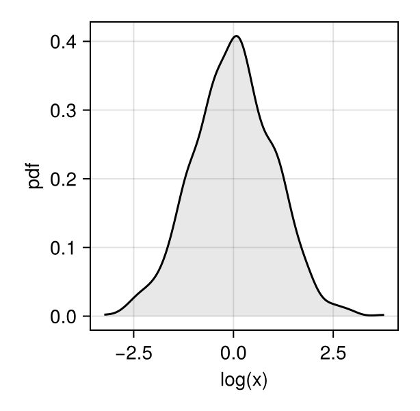
The two plots look different. The first represents the pdf of x in a log scale, while the second represents the pdf of log(x) in a linear scale. The two curves differ by a factor 1 / x, the derivative of log(x). See e.g. this post for some mathematical background on the topic.
In general, the second approach (plotting the density of log(x)) could be considered more principled, as it preserves the proportionality between area and probability mass. On the contrary, the first approach (plotting the density of x in a log scale) breaks this proportionality relationship.
A similar reasoning applies to histograms:
using AlgebraOfGraphics
df = (x = exp.(rand(1000)),)
hist1 = data(df) * mapping(:x) * histogram()
draw(hist1, axis=(width=225, height=225, xscale=log))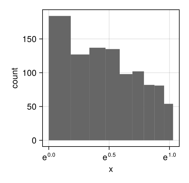
df = (x = exp.(rand(1000)),)
hist2 = data(df) * mapping(:x => log => "log(x)") * histogram()
draw(hist2, axis=(width=225, height=225))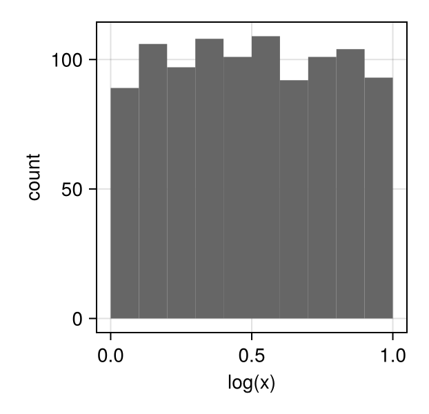
The data transformation approach is preferable as it produces uniform bins, which are easier to interpret.
How to combine AlgebraOfGraphics with plain Makie plots?
Since AlgebraOfGraphics is built upon the Makie ecosystem we can easily combine plots from both packages. Two approaches can be taken. Firstly, by using draw! you can pass a Figure or FigurePosition created by Makie to be used by AlgebraOfGraphics, e.g.
f, a, p = lines(0..2pi, sin; figure = (size = (600, 400),))

df = (x = exp.(rand(1000)),)
hist1 = data(df) * mapping(:x => log => "log(x)") * histogram()
draw!(f[1, 2], hist1)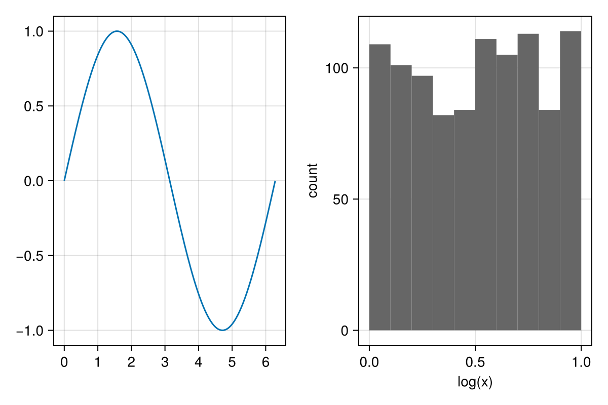
Alternatively, we can create the AlgebraOfGraphics figure first and then add in additional plain Makie axes alongside the result by accessing the .figure field of fg, e.g.
df = (x = exp.(rand(1000)),)
hist2 = data(df) * mapping(:x => log => "log(x)") * histogram()
fg = draw(hist2; figure = (size = (600, 400),))

lines(fg.figure[1, 2], 0..2pi, cos)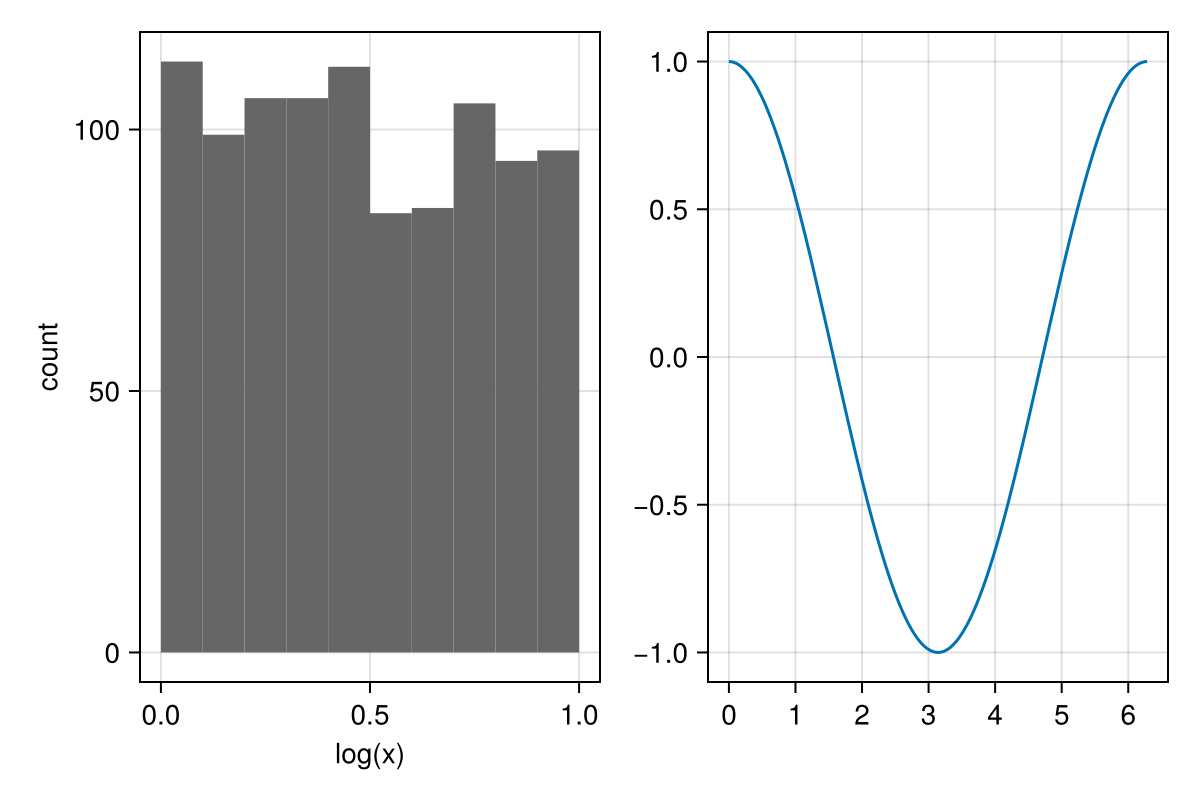
Note
When setting the width and height dimensions of each axis manually you will need to call resize_to_layout!(fg) before displaying the figure such that each axis is sized correctly.